GSEA在我脑中一直是一个比较耗时,而且也消耗内存的工作。很多年之前果子老师,让我帮他写并行代码,进行GSEA分析,然后我发现当时的128G内存不够,溢出了。
最近我突然想到,能不能再python中做GSEA分析呢?于是我搜了下,发现还真有!名字叫GSEApy, 对应文章是”Zhuoqing Fang, Xinyuan Liu, Gary Peltz, GSEApy: a comprehensive package for performing gene set enrichment analysis in Python,
Bioinformatics, 2022;, btac757, https://doi.org/10.1093/bioinformatics/btac757“,也是刚发表不到1年。
GSEA是描述基因表达变化的常用算法。然而,目前用于执行 GSEA 的工具分析大型数据集的能力有限,这在分析单细胞数据时尤其成问题。为了克服这一局限,我们用 Python 开发了一个 GSEA 软件包(GSEApy),它可以高效地分析大型单细胞数据集。 GSEA。GSEApy 使用 Rust 实现,能够计算与 GSEA 相同的路径集合富集统计量。GSEApy 的 Rust 实现比 GSEApy 的 Numpy 版本(v0.10.8)快 3 倍,内存使用量少 4 倍以上
更为惊喜的是,我发现这个GSEApy的底层实现居然还是Rust,一门高性能的编程语言,那么到底速度如何呢?我用的果子老师的数据,做了测试。
如下是R版本的代码
### GSEA 分析
load(file = "./DEseq2_ESR1_Diff.Rdata")
library(dplyr)
gene_df <- res %>%
  dplyr::select(gene_id,logFC,gene) %>%
  ## 去掉NA
  filter(gene!="") %>%
  ## 去掉重复
  distinct(gene,.keep_all = T)

### 1.获取基因logFC
geneList <- gene_df$logFC
### 2.命名
names(geneList) = gene_df$gene
## 3.排序很重要
geneList = sort(geneList, decreasing = TRUE)

head(geneList)
library(clusterProfiler)

### GSEA 分析

start_time <- Sys.time()
hallmarks <- read.gmt("./h.all.v7.1.symbols.gmt")
gseahallmarks <- GSEA(geneList,TERM2GENE =hallmarks)
# 获取程序结束时间
end_time <- Sys.time()

# 计算程序执行时间
execution_time <- end_time - start_time

# 输出程序执行时间
print(execution_time)
# Time difference of 24.17011 secs
接着,我们试试python版本的GSEA,首先要安装GSEA
pip install gseapy
代码如下,其中geneList是让GPT模仿R版本的预处理代码编写,gp.prerank是我修改自官方教程
import pandas as pd

# Assuming you have a DataFrame called 'res' in Python
# that corresponds to your 'gene_df' in R
res = pd.read_csv("E:/gsea_analysis/DEseq2_ESR1_Diff.csv")
# Select the columns 'gene_id', 'logFC', and 'gene'
gene_df = res[['gene_id', 'logFC', 'gene']]

# Filter out rows where 'gene' is not empty,NaN
gene_df = gene_df[gene_df['gene'].isnull() == False]

# Remove duplicates based on the 'gene' column
gene_df = gene_df.drop_duplicates(subset=['gene'], keep='first')

# 1. Get the 'logFC' values into a list
geneList = gene_df['logFC']
geneList.index = gene_df['gene']
geneList = geneList.sort_values(ascending=False)


start_time = time.time()
pre_res = gp.prerank(rnk= geneList , # or rnk = rnk,
                     gene_sets= "E:/gsea_analysis/h.all.v7.1.symbols.gmt",
                     threads=1,
                     min_size=5,
                     max_size=1000,
                     permutation_num=1000, # reduce number to speed up testing
                     outdir=None, # don't write to disk
                     seed=6,
                     verbose=True, # see what's going on behind the scenes
                    )
# Record the end time
end_time = time.time()

# Calculate and print the execution time
execution_time = end_time - start_time
print("Execution Time: {:.2f} seconds".format(execution_time))

# Execution Time: 2.13 seconds
从速度来说,R版本用了24秒,而gseapy只用了2秒多一点,几乎快了10倍多!那么结果一样吗?
我分析了下,稍微还是有一些区别,但是不大。在gseapy的输出结果中,NOM p-val<0.05的结果有22条,R版本的GSEA结果是20条,当然gseapy的22条都在GSEA中出现,但几乎可以忽略不计了!
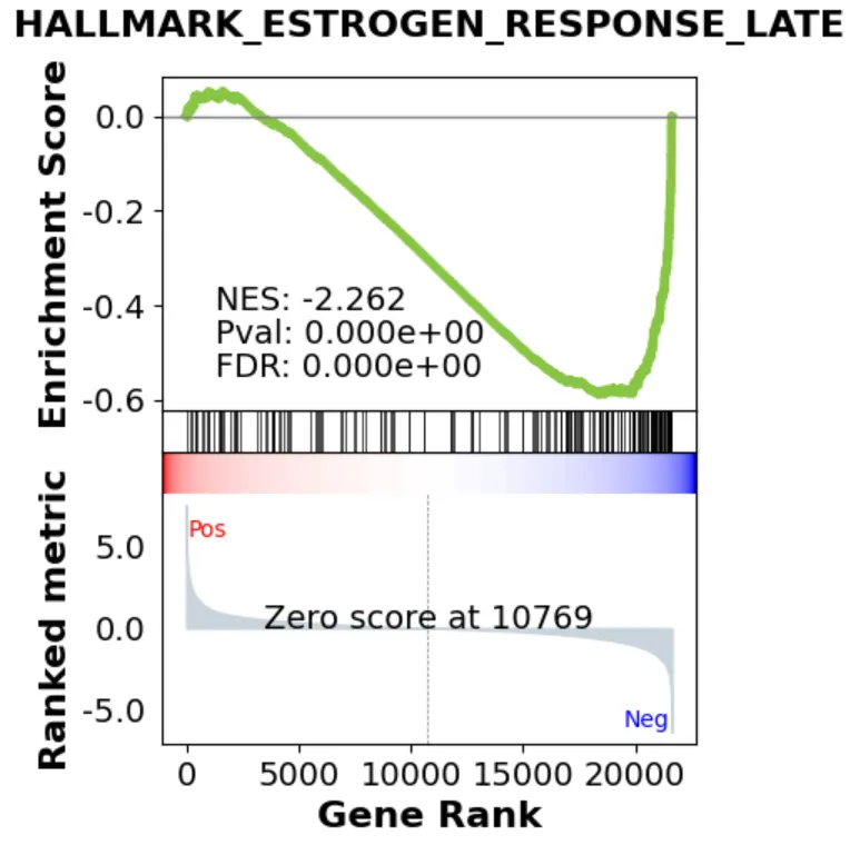
gseapy提供了一些画图函数,可以用来展示结果,比如说,我们需要绘制最常见的GSEA的结果图。
term = "HALLMARK_ESTROGEN_RESPONSE_LATE"
axs = pre_res.plot(terms= term, show_ranking=True) # v1.0.5
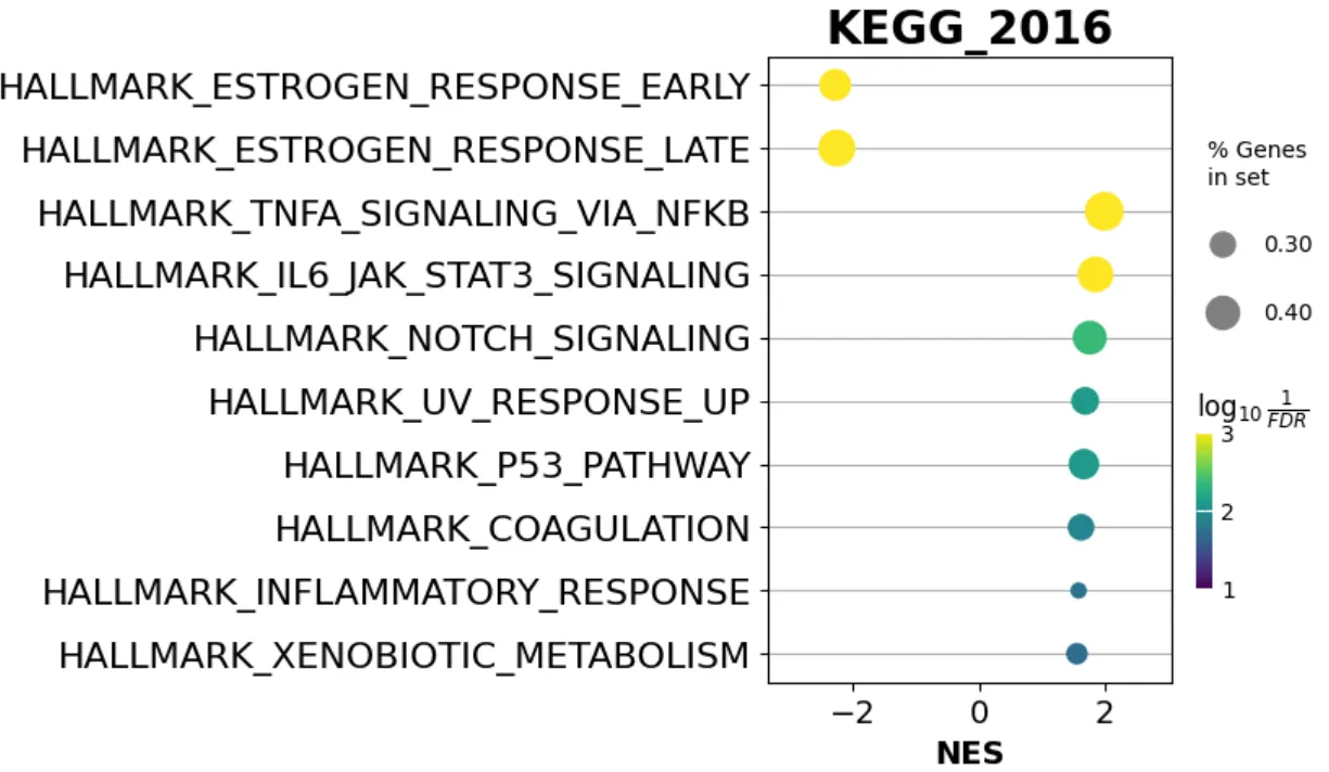
亦或者想看点图结果
import matplotlib.pyplot as plt
from gseapy import dotplot
# to save your figure, make sure that ``ofname`` is not None
ax = dotplot(pre_res.res2d,
             column="FDR q-val",
             title='KEGG_2016',
             cmap=plt.cm.viridis,
             size=6, # adjust dot size
             figsize=(4,5), cutoff=0.25, show_ring=False)
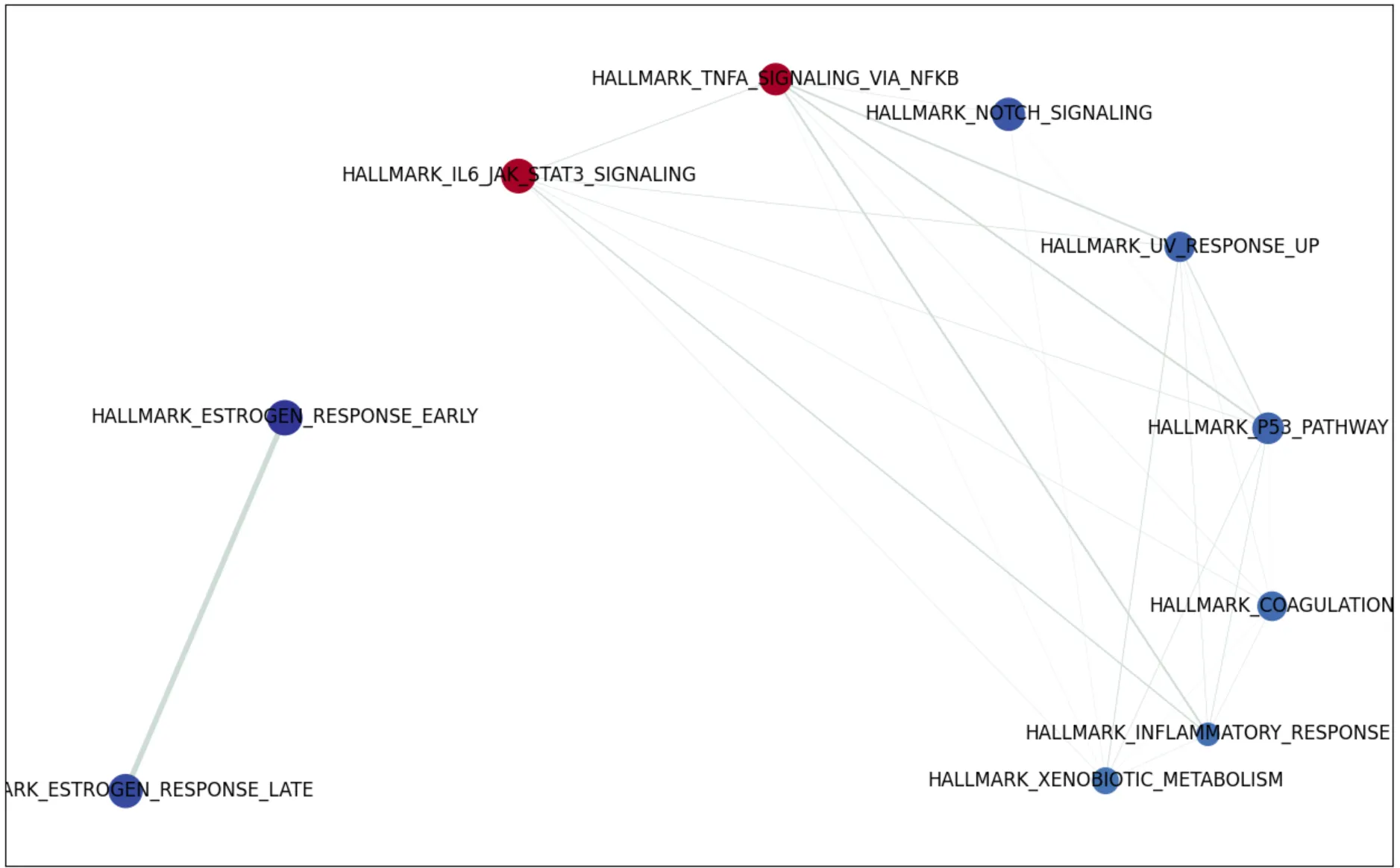
亦或者是网络图
from gseapy import enrichment_map
import networkx as nx

nodes, edges = enrichment_map(pre_res.res2d)
G = nx.from_pandas_edgelist(edges,
                            source='src_idx',
                            target='targ_idx',
                            edge_attr=['jaccard_coef', 'overlap_coef', 'overlap_genes'])

fig, ax = plt.subplots(figsize=(16, 10))

# init node cooridnates
pos=nx.layout.spiral_layout(G)
#node_size = nx.get_node_attributes()
# draw node
nx.draw_networkx_nodes(G,
                       pos=pos,
                       cmap=plt.cm.RdYlBu,
                       node_color=list(nodes.NES),
                       node_size=list(nodes.Hits_ratio *1000))
# draw node label
nx.draw_networkx_labels(G,
                        pos=pos,
                        labels=nodes.Term.to_dict())
# draw edge
edge_weight = nx.get_edge_attributes(G, 'jaccard_coef').values()
nx.draw_networkx_edges(G,
                       pos=pos,
                       width=list(map(lambda x: x*10, edge_weight)),
                       edge_color='#CDDBD4')
plt.show()
但是,假设,你更偏好于用R进行可视化,比如说用Y叔开发的 enrichplot 画图,所以我写了一小段代码,输出结果,用于cluterProfiler画图。
首先,将GSEApy的结果保存成csv, 一个排序信息,一个是GSEA运行结果
pre_res.ranking.to_csv("./geneList.csv")
pre_res.res2d.to_csv("./gseapy.csv", index=False)
然后在R语言中,我们读取保存的文件,然后自己用new创建一个gseaResult,只不过数据来自于GSEApy
df <- read.csv("./gseapy.csv")

# 读取gene排序
geneList_df <- read.csv("./geneList.csv")
geneList <- geneList_df$prerank
names(geneList) <- geneList_df$gene_name

# hallmarks ,也就似乎基因集信息
hallmarks <- read.gmt("./h.all.v7.1.symbols.gmt")
gene_sets <- split(hallmarks$gene, hallmarks$term)


# 输出结果的result
result <- data.frame(
  "ID" = df$Term ,
  "Description"= df$Term ,
  "setSize"= sapply(strsplit(df$Tag.., "/"), function(x) as.numeric(x[2])),
  "enrichmentScore"=df$ES,
  "NES"= df$NES,
  "pvalue"= df$NOM.p.val,
  "p.adjust"=df$FDR.q.val,
  "qvalue"=df$FWER.p.val,
  "rank"= 1,
  "leading_edge"= "",
  "core_enrichment" = gsub(";","/",df$Lead_genes)
)

rownames(result) <- result$ID
# 需要注意的是params,我设置了pvalueCutoff=1, 因为没有限制。
my_result <- new("gseaResult", result = result,
                 geneSets=gene_sets,
                 geneList=geneList,
                 params = list(pvalueCutoff = 1,  exponent = 1, minGSSize=10, maxGSSize=500)
                 )
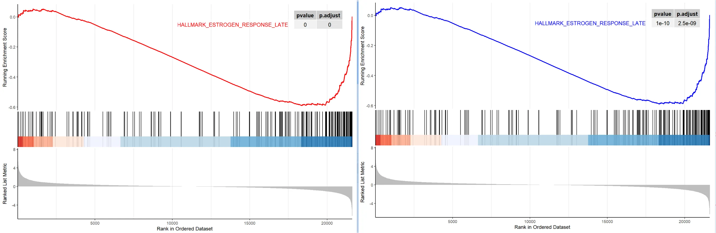
于是乎,神奇的事情就发生了,我们可以用 enrichplot 包的函数画图了!
library(enrichplot)

pathway.id = "HALLMARK_ESTROGEN_RESPONSE_LATE"
p1 <- gseaplot2(my_result,
          color = "red",
          geneSetID = pathway.id,
          pvalue_table = T)

p2 <- gseaplot2(gseahallmarks,
          color = "blue",
          geneSetID = pathway.id,
          pvalue_table = T)
自此,鱼与熊掌兼得